Marvelous Tips About How To Draw Charts In Ms Excel
/ExcelCharts-5bd09965c9e77c0051a6d8d1.jpg)
How To Create A Chart In Excel Using Shortcut Keys
/ExcelCharts-5bd09965c9e77c0051a6d8d1.jpg)
How To Create A Chart In Excel Using Shortcut Keys
Excel Quick And Simple Charts Tutorial - Youtube
Video: Create A Chart
How To Create Charts In Excel (in Easy Steps)
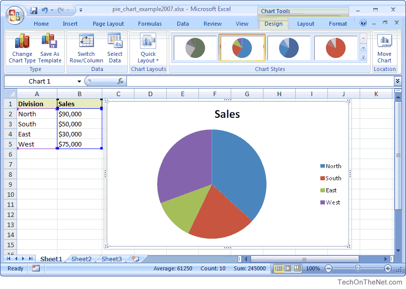
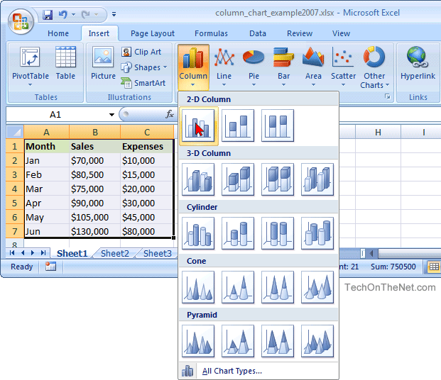
Ms Excel 2007: How To Create A Pie Chart
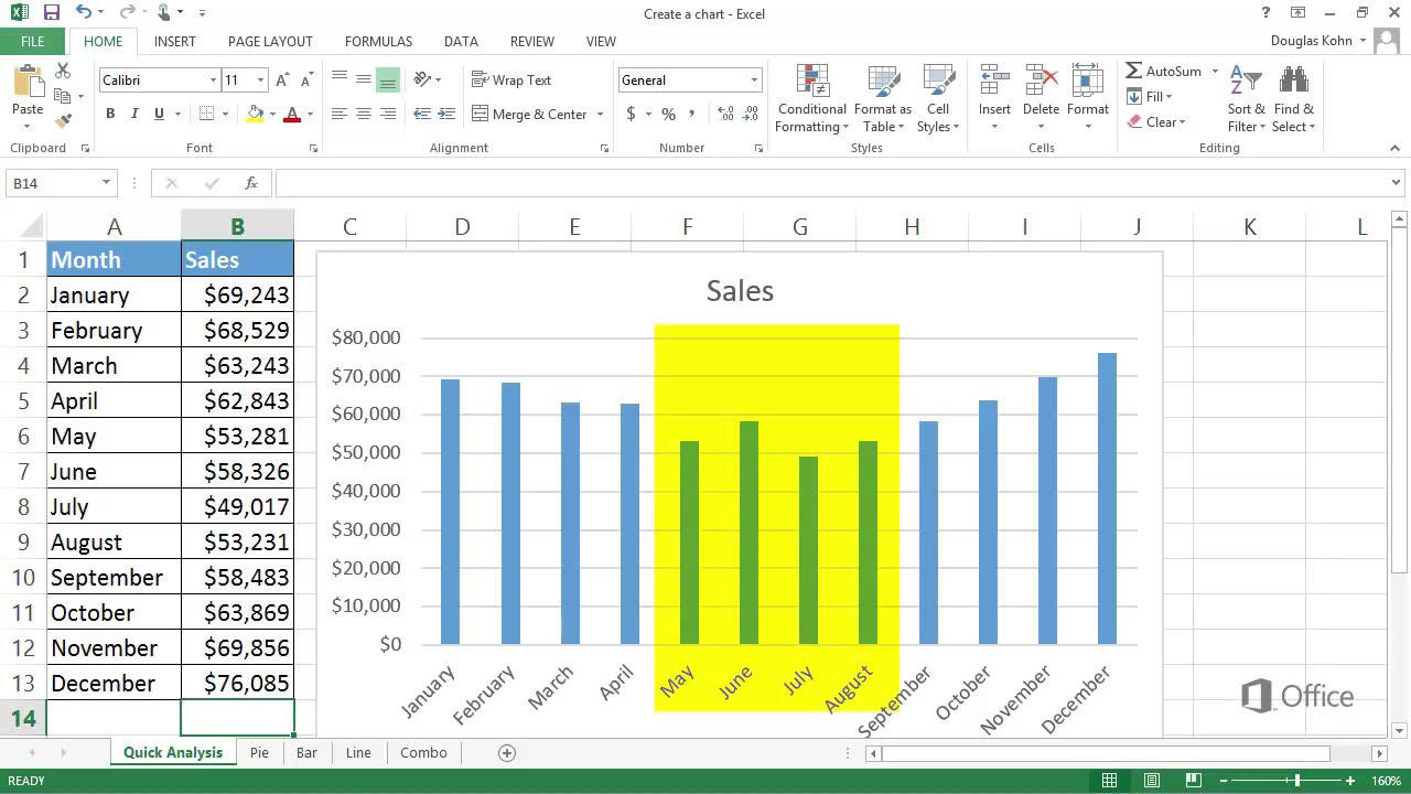
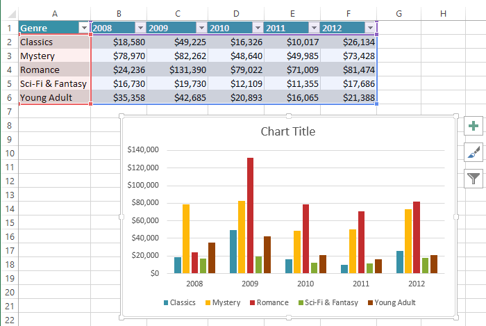
Excel creates graphs which can display data clearly.
How to draw charts in ms excel. To create a pivot table using our ledger data, navigate to the insert tab. Click on the pivottable option and click from table/range in the dropdown menu. Now, in the charts group, you need to click on the “insert pie or doughnut chart” option.
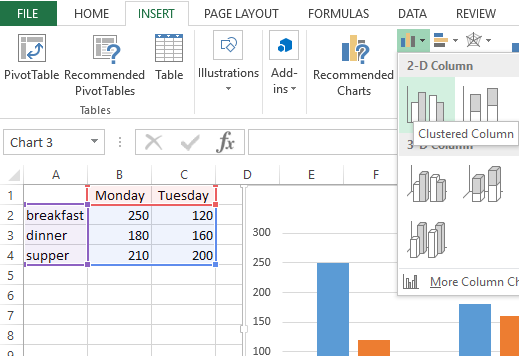
Go to insert and click on bar chart and select the first chart. This is how you can plot a simple graph using microsoft excel. Do not select the sum of any numbers as you probably don’t want to display it on your chart.
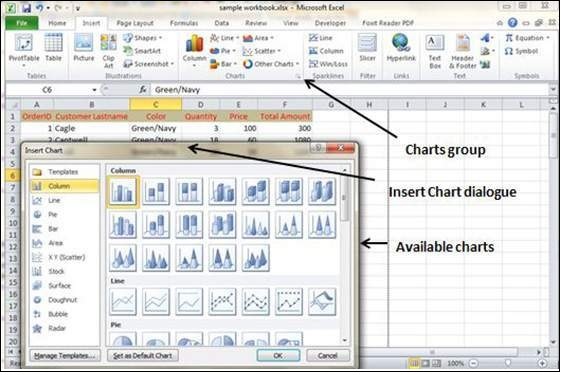
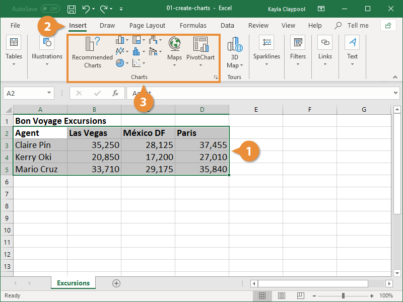
Select the data for your chart and go to the insert tab. Insert a smartart (shape) first, create a blank new worksheet. The type of excel charts covered are column, bar, line and a com.
This video tutorial will show you how to create a chart in microsoft excel. Ad explore different types of data visualizations and learn tips & tricks to maximize impact. Click on the insert tab.
Learn the basics of excel charts to be able to quickly create graphs for your excel reports. Learn more about different chart and graph types with tableau's free whitepaper. Learn at your own pace.
Select the illustration group and insert a smartart in your excel. To do so, select the entire data set b2:d16 and do the following: Excel for the web allows you to view power pivot tables and charts, but you need the excel desktop app to create power pivot data models.
This method is a somewhat advanced way of creating a comparison chart. Learn how to add a linear trendline and an equation to your graph in excel. Learn the steps involved in.
By using pivot table and line. Applying pivot table and line chart to create a comparison chart. Once you click on the chart, it will insert the chart as shown in the below image.
In your spreadsheet, select the data that you want to plot on your pie chart.
Ms Excel 2007: How To Create A Column Chart
Simple Charts In Excel 2010
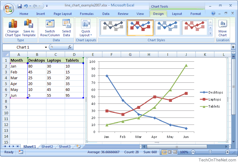
Ms Excel 2007: How To Create A Line Chart
Drawing Of Charts And Diagrams In Excel
/format-charts-excel-R1-5bed9718c9e77c0051b758c1.jpg)
Make And Format A Column Chart In Excel

How To Make A Bar Chart In Microsoft Excel
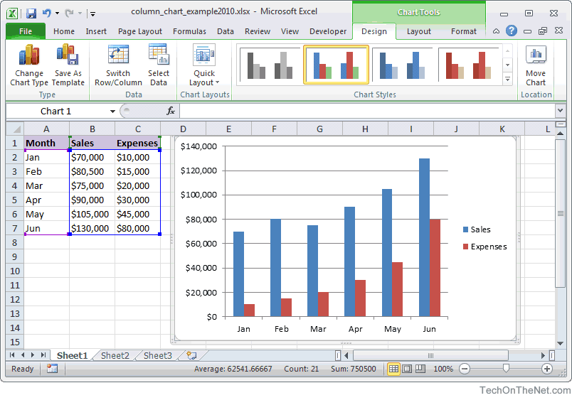
Ms Excel 2010: How To Create A Column Chart
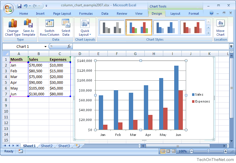
Ms Excel 2007: How To Create A Column Chart
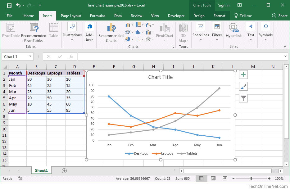
Ms Excel 2016: How To Create A Line Chart
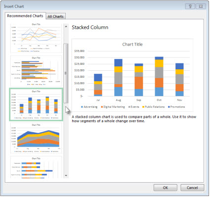
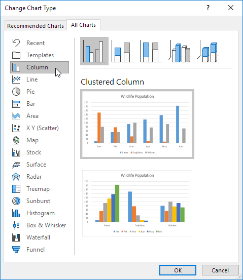
Create A Chart With Recommended Charts
Excel 2013: Charts

How To Create Dynamic Charts In Ms Excel (tamil) | Get Update Automatically - Youtube
How To Make A Chart Or Graph In Excel | Customguide
